Simple Walkthrough

This is intended as a basic example of using the imexam package as a quicklook for image examination. If you are new to python or to the python version of imexam, start here to get your feet wet.

First you need to import the package

import imexam

Usage with D9 (the current default viewer)

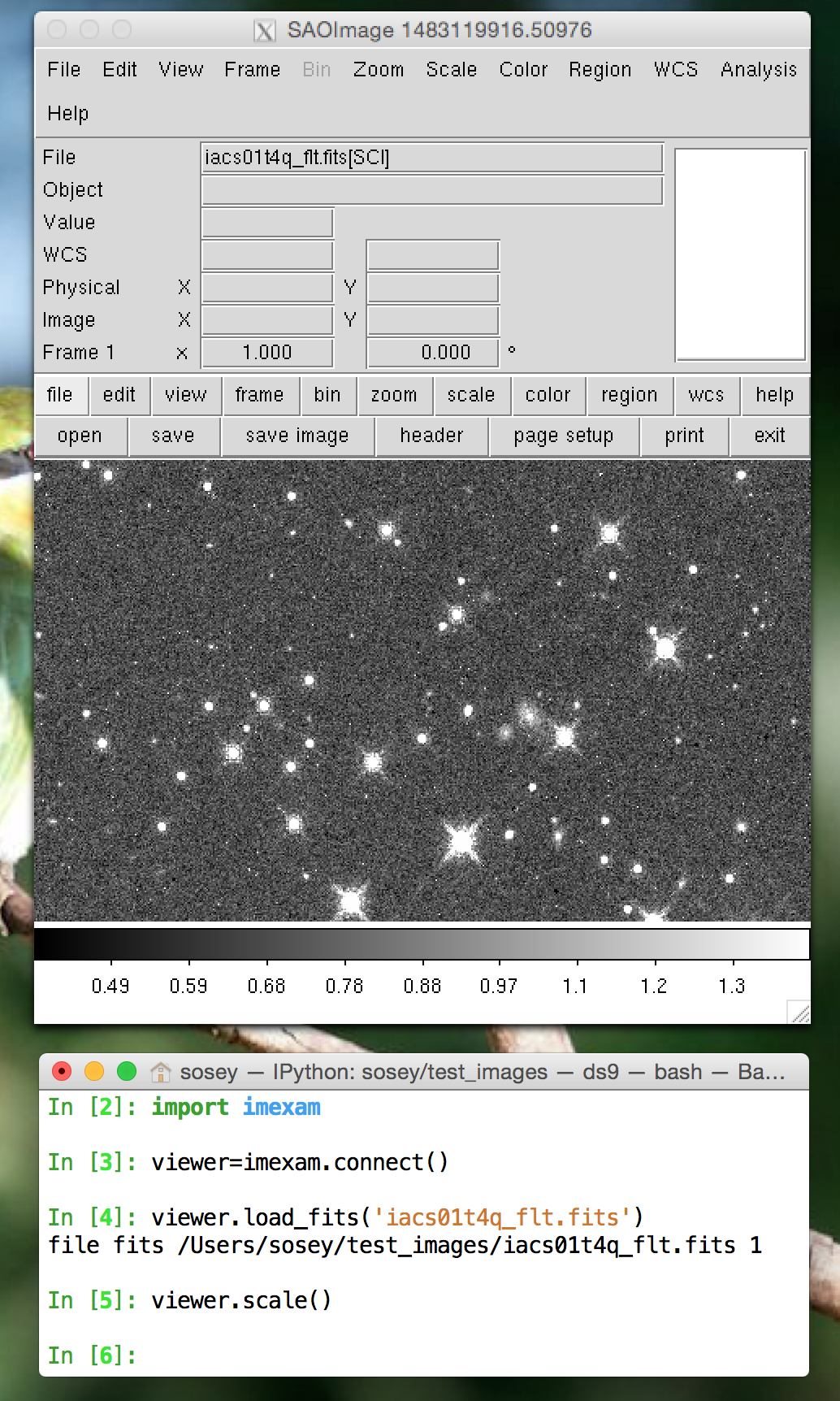
Start up a DS9 window (DS9 is the default viewer):

• a new DS9 window will be opened

• open a fits image

• scale the image using zscale():

  viewer=imexam.connect()  # startup a new DS9 window
  viewer.load_fits('iacs01t4q_flt.fits')  # load a fits image into it
  viewer.scale()  # run default zscaling on the image
  

If you already have a DS9 gui running, you can ask for a list of available windows:

# This will display if you've used the default command above and have no other DS9 windows open
In [1]: imexam.list_active_ds9()
DS9 imexam1522943947.288667 gs a825364:62436 sosey
Out[2]: {'a825364:62436': ('imexam1522943947.288667', 'sosey', 'DS9', 'gs')}

## imexam puts its own unique name on the window

# open a window in another process from the shell
# you should see it use the default name, 'ds9'
In [3]: !ds9&
In [4]: imexam.list_active_ds9()
Out[7]:
{'a825364:62436': ('imexam1522943947.288667', 'sosey', 'DS9', 'gs'),
 'a825364:62459': ('ds9', 'sosey', 'DS9', 'gs')}

You can attach to a current DS9 window by specifying its unique name, this is the first name listed in the dictionary item values tuple:

viewer1 = imexam.connect('ds9')

If you haven’t given your windows unique names using the -title <name> option from the commandline, then you must use the ip:port address. This address is also the key that is returned in the dictionary of active DS9 windows. In order to attached to the window we stared in the shell, use : a825364:62459

viewer1 = imexam.connect(‘a825364:62459’)

Load a fits image into the new DS9 window:

viewer1.load_fits(‘n8q624e8q_cal.fits’)

You may have noticed that the information from list_active_ds9() is returned in a python dictionary structure, this is to enable quick cycling or picking of available DS9 windows by asking for the keys in the dictionary. This following is just for instruction purposes, the code below asks for the list of windows and then successively displays the same image to each one:

ds9_windows = imexam.list_active_ds9()
for window in ds9_windows:
    temp=imexam.connect(window)
    temp.load_fits('n8q624e8q_cal.fits')

It’s also possible to load a FITS image object that you already have opened in your python session, if no extension is given, then the first IMAGE exension that is found will be loaded as a numpy array:

from astropy.io import fits
image = fits.open('n8q624e8q_cal.fits')
viewer1.load_fits(image)

Using get_viewer_info() returns information about what is contained inside the DS9 window. There could be many uses for the returned dictionary, here I’m just listing the information to show you how the display of the FITS file versus the FITS object changes the information that imexam stores:

In [23]: viewer1.get_viewer_info()
Out[23]:
{'1': {'extname': 'SCI',
  'extver': 1,
  'filename': '/Users/sosey/test_images/n8q624e8q_cal.fits',
  'iscube': False,
  'mef': True,
  'naxis': 0,
  'numaxis': 2,
  'user_array': None}}

  # Above, you can see there is only 1 frame, named 1, that
  # contains a multi-extension fits file

In [24]: from astropy.io import fits
In [25]: image = fits.open('n8q624e8q_cal.fits')
In [26]: viewer1.load_fits(image)
In [27]:  viewer1.get_viewer_info()
Out[27]:
{'1': {'extname': None,
  'extver': None,
  'filename': None,
  'iscube': False,
  'mef': False,
  'naxis': 0,
  'numaxis': 2,
  'user_array': array([[ 0.        ,  0.        ,  0.73420113, ...,  2.29928851,
           1.13779497,  0.40814143],
         [ 0.        ,  0.76415622,  0.        , ...,  2.02307796,
           1.07565212,  0.44265628],
         [ 0.        ,  0.76297635,  0.65969932, ...,  0.61184824,
           0.48248726,  0.41064522],
         ...,
         [ 0.5144701 ,  0.38698068,  0.31468284, ...,  1.57044649,
           0.42518842,  0.50868863],
         [ 0.44805121,  0.34715804,  0.33939072, ...,  0.67747742,
           0.46475834,  0.51104462],
         [ 0.53063494,  0.54570055,  0.53724855, ...,  0.4361479 ,
           0.58057427,  0.45152891]], dtype=float32)}}

  # Above you can see that there is only 1 frame, but it contains
  # a numpy array and no filename reference.

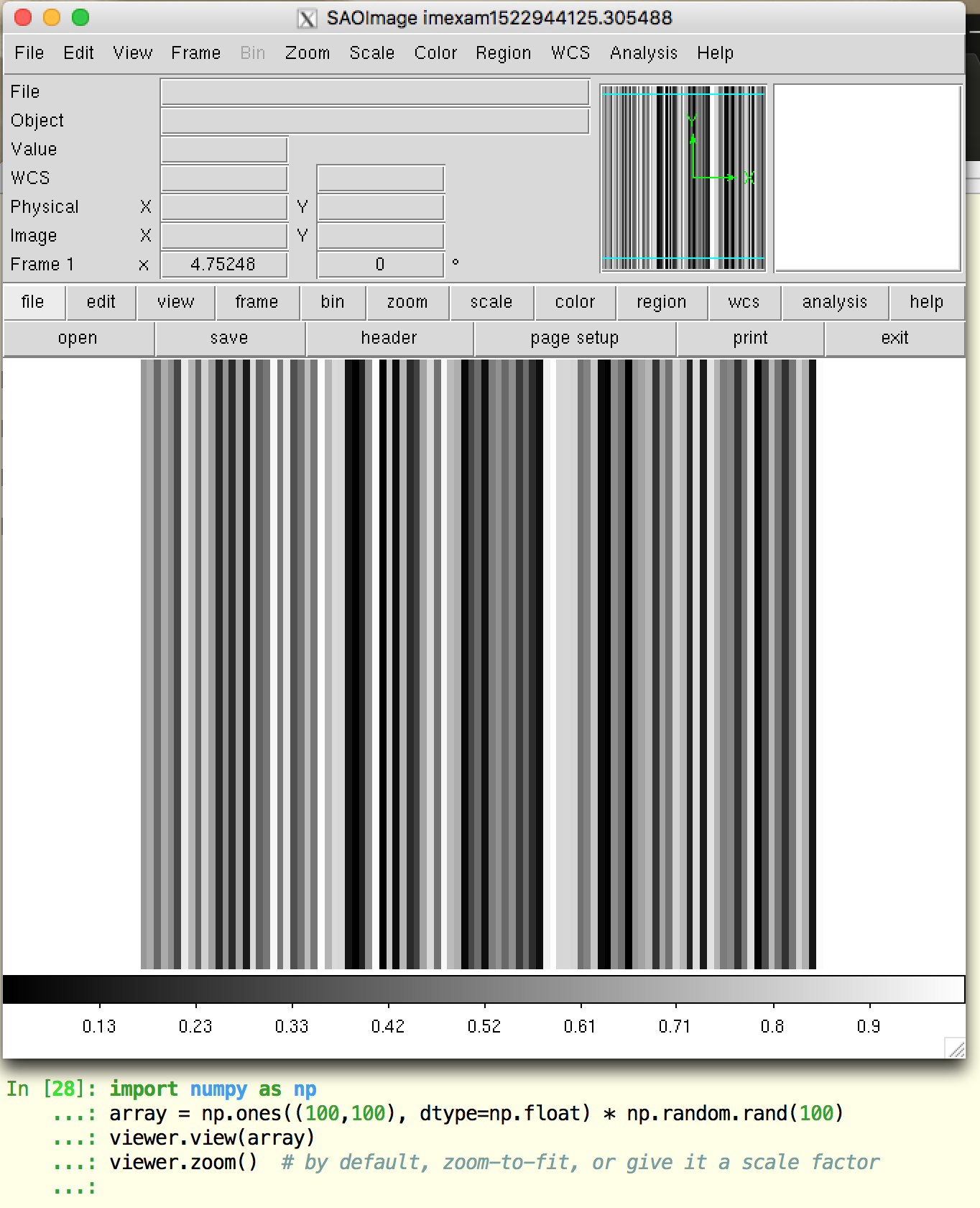
You can also load a numpy array directly, we’ll create an example array and display it to our viewer:

import numpy as np
array = np.ones((100,100), dtype=np.float) * np.random.rand(100)
viewer.view(array)
viewer.zoom()  # by default, zoom-to-fit, or give it a scale factor

Now lets use imexam() to create a couple plots:

viewer.load_fits('n8q624e8q_cal.fits')
viewer.imexam()

The available key mappings should be printed to your terminal:

In [7]: viewer.imexam()

Press 'q' to quit

2   Make the next plot in a new window
a   Aperture sum, with radius region_size
b   Return the 2D gauss fit center of the object
c   Return column plot
e   Return a contour plot in a region around the cursor
g   Return curve of growth plot
h   Return a histogram in the region around the cursor
j   1D [Gaussian1D default] line fit
k   1D [Gaussian1D default] column fit
l   Return line plot
m   Square region stats, in [region_size],default is median
r   Return the radial profile plot
s   Save current figure to disk as [plot_name]
t   Make a fits image cutout using pointer location
w   Display a surface plot around the cursor location
x   Return x,y,value of pixel
y   Return x,y,value of pixel

Look at the window below, I’ve started the imexam loop and then pressed the ‘a’ key to create an aperture photometry plot (which also printed information about the photometry to the terminal), then I pressed the ‘2’ key in order to keep the current plot open and direct the next plot to a new window, where I’ve asked for a line plot of the same star, using the ‘l’ key.

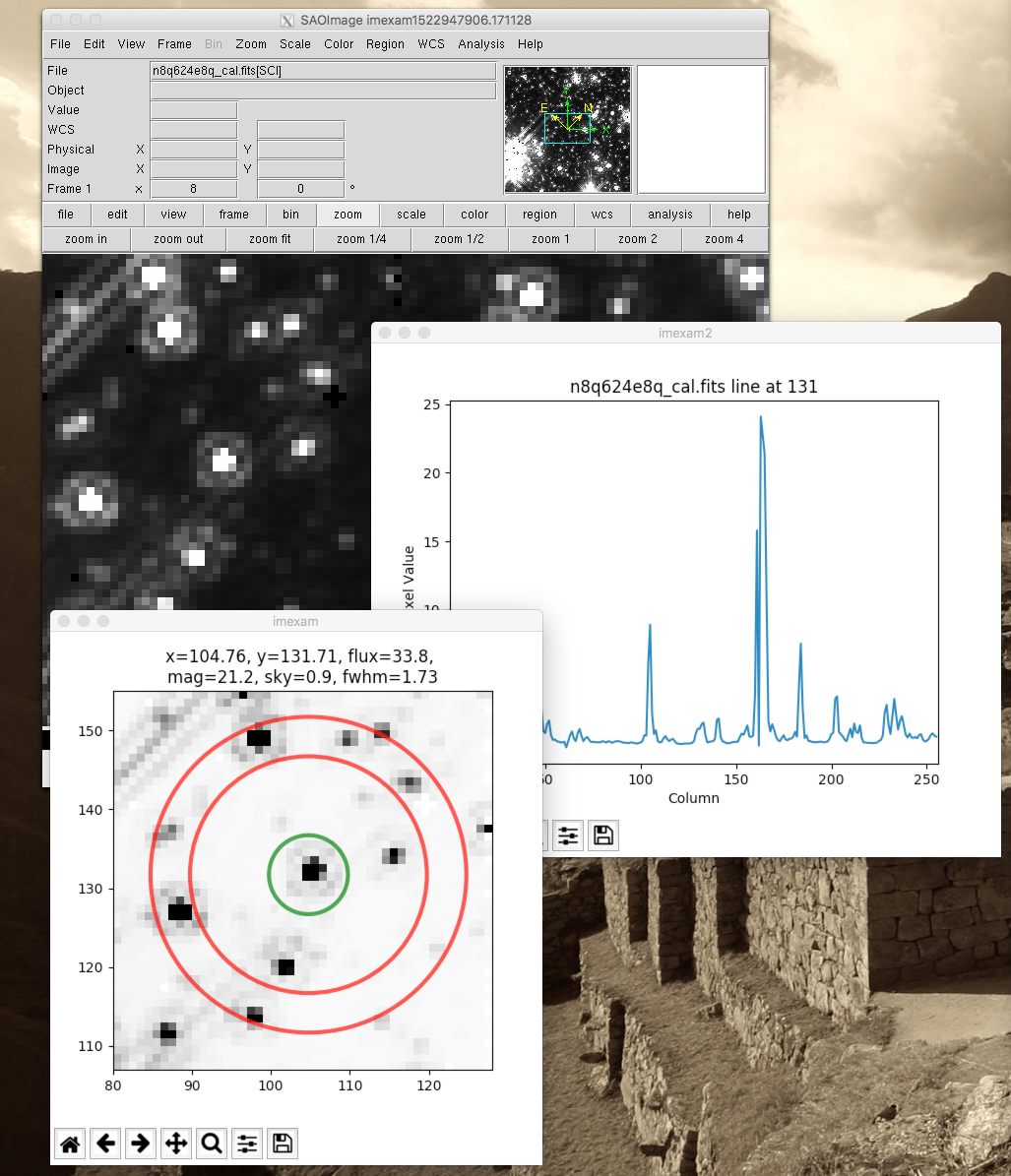
You should see the printed information in your terminal:

Current image /Users/sosey/test_images/n8q624e8q_cal.fits
xc=104.757598   yc=131.706727
x              y              radius         flux           mag(zpt=25.00) sky/pix        fwhm(pix)
104.76         131.71         5              33.84          21.18          0.87           1.73
Plots now directed towards imexam2
Line at 104.75 131.625

Users may change the default settings for each of the imexamine recognized keys by editing the associated dictionary. You can edit it directly, by accessing each of the values by their keyname and then reset mydict to values you prefer. You can also create a new dictionary of functions which map to your own analysis functions.

However, you can access the same dictionary and customize the plotting parameters using set_plot_pars. In the following example, I’m setting three of the parameters for the contour map, whose imexam key is “e”:

#customize the plotting parameters (or any function in the imexam loop)
viewer.set_plot_pars('e','title','This is my favorite galaxy')
viewer.set_plot_pars('e','ncontours',4)
viewer.set_plot_pars('e','cmap','YlOrRd') #see http://matplotlib.org/users/colormaps.html

where the full dictionary of available values can be found using the eimexam() function described above.:

In [1]: viewer.eimexam()
Out[2]:
{'ceiling': [None, 'Maximum value to be contoured'],
 'cmap': ['RdBu', 'Colormap (matplotlib style) for image'],
 'floor': [None, 'Minimum value to be contoured'],
 'function': ['contour'],
 'label': [True, 'Label major contours with their values? [bool]'],
 'linestyle': ['--', 'matplotlib linestyle'],
 'ncolumns': [15, 'Number of columns'],
 'ncontours': [8, 'Number of contours to be drawn'],
 'nlines': [15, 'Number of lines'],
 'title': [None, 'Title of the plot'],
 'xlabel': ['x', 'The string for the xaxis label'],
 'ylabel': ['y', 'The string for the yaxis label']}

Users may also add their own imexam keys and associated functions by registering them with the register(user_funct=dict()) method. The new binding will be added to the dictionary of imexamine functions as long as the key is unique. The new functions do not have to have default dictionaries association with them, but users are free to create them.

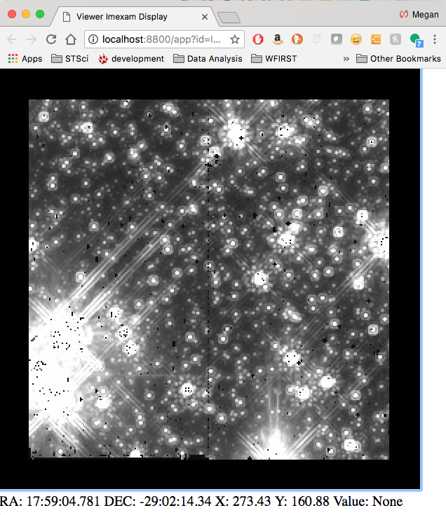
Usage with Ginga viewer

Start up a ginga window using the HTML5 backend and display an image. Make sure that you have installed the most recent version of ginga, imexam may return an error that the viewer cannot be found otherwise.:

# since we've already used the viewer object
# to point to a DS9 window in the example
# above, we'll first cleanly close that down
viewer.close()

# now connect to a ginga window
viewer=imexam.connect(viewer='ginga')
viewer.load_fits('n8q624e8q_cal.fits')

Note

All commands after your chosen viewer is opened are the same. Each viewer may also have it’s own set of commands which you can additionally use.

Scale the image to the default scaling, which is a zscale algorithm, but the viewers other scaling options are also available:

viewer.scale()
viewer.scale('asinh')  # <-- uses asinh

Note

When using the Ginga interface, the imexam plotting and analysis functions are used by pressing the ‘i’ key to enter imexam mode. Inside this mode the key mappings are as listed by imexam, outside of this mode (pressing ‘q’) the Ginga key mappings are in effect.

When you are using the HTML5 Ginga viewer, the close() method will stop the HTTP server, but you must close the window manually.

In [34]: viewer.close() Stopped http server